
Transformer Quality in Linear Time
0. Abstract
Transformers의 디자인을 분석하여, “Long-sequences” 약점을 해결할 수 있는 방법들을 제안합니다.
- 첫 번째로 gated attention unit라는 간단한 layer를 제안합니다. 품질 감소를 최소화 하면서도 약소한 single-head attention을 쓸 수 있습니다.
- 다음으로 a linear approximation method를 제안합니다. accelerator-friendly하며, 품질 측면에서 우수합니다.
1. Introduction
Transformers는 딥러닝의 새로운 SOTA engine이 됐으며, Language와 vision 모두에서 새로운 단계로의 돌파구가 됐습니다. 모델 크기가 점점 증가해왔으나, 대부분의 Transformers는 short context size에 한정돼있습니다. input 길이에 따라 지수적으로 복잡도가 증가하기 때문입니다. 이러한 한계는 Transformers가 long-term information을 처리할 수 없게 만드는 요인입니다.
다양한 기법들이 context 길이를 확장한 Transformers의 속도 향상에 attention 기법의 개선으로 도전했습니다.
- Child et al., 2019
- Dai et al., 2019
- Rae et al., 2019
- Choromanski et al., 2020
- Wang et al., 2020
- Katharopoulos et al., 2020
- Beltagy et al., 2020
- Zaheer et al., 2020
- Kitaev et al., 2020
- Roy et al., 2021
- Jaegle et al., 2021
이전의 많은 노력에도 불구하고 SOTA 시스템에서는 기본 Transformers가 여전히 주류 디자인인 상태입니다. 본 논문에서 이 이슈를 실무적 관점에서 연구해보고, 다음과 같은 단점들을 극복할 수 있는 효율적인 attention 방법을 찾아봅니다.
Inferior Quality
vanilla Transformers가 몇몇 간단한 augmentation을 적용한다면, 지금까지 제안된 방법들보다 훨씬 더 좋은 성능을 보인다는 것을 확인했습니다. “efficient attention” 방법들은 단순 augmented Transformers 대비 심각한 품질 저하를 보여줬고, 이는 효율성에서 얻는 효용보다 더 큰 문제입니다.
Overhead in Practice
지금까지의 “efficient attention”은 Transformer layers를 복잡하게 하고, 막대한 data/memory formatting 연산들이 필요합니다. 그래서 GPU/TPU를 사용함에 있어 실제 복잡도와 이론적 복잡도의 큰 차이가 존재합니다.
Inefficient Auto-regressive Training
대부분의 attention 선형화 기법들은 inference 할 때는 빠르지만, language 모델 등을 auto-regressive하게 학습할 때는 굉장히 느립니다. 이것은 RNN 스타일의 sequential state updating 때문입니다. 이러한 방법은 최신 가속기(GPU/TPU)를 제대로 활용할 수 없습니다.
본 논문에서 최초로 fully augmented Transformers의 품질을 유지하면서도 진정한 의미의 context linear scalability를 달성했습니다. 지금까지의 “efficient attention” 방법론들은 Transformers의 multi-head self-attention (MHSA)를 직접 근사하려 했습니다. 그러나 저자들은 더 뛰어난 품질을 근사할 수 있는 새로운 layer를 디자인했습니다. 본 논문에서 제안하는 모델인 FLASH(Fast Linear Attention with a Single Head)는 두 단계로 구성됩니다.
먼저, “effective approximation”에 더욱 적합한 새로운 layer를 제안합니다. gating mechanism을 도입하여 self-attention의 부담을 덜어낼 수 있는 Gated Attention Unit (GAU)를 고안했습니다. GAU layer는 Transformer layers보다 경제적이며, 무엇보다 Attention의 정밀함을 덜 요구한다는 점이 중요합니다.
small single-head가 달려있는 softmax-free attention인 GAU는 Transformers처럼 동작합니다. GAU도 역시 context size에 따라 지수적으로 복잡도가 증가하지만, attention의 역할을 줄임으로써 품질 저하를 막으면서도 근사 기법들을 사용할 수 있는 것입니다.
그 다음 GAU에서 quadratic attention를 근사할 수 있는 효율적인 방법들을 소개합니다. 이로써 context size에 따라 복잡도가 선형적으로 증가하는 효과를 얻을 수 있는 것입니다.
핵심 아이디어는 first group tokens를 cunks로 만드는 것이며, chunk 내에서는 기존 quadratic attention을 chunks 끼리는 fast linear attention을 사용하는 것입니다.
2. Gated Attention Unit
Vanilla MLP
Let $X \in \mathbb{R}^{T \times d}$ be the representation over T tokens.
Transformer’s MLP 결과는 $O = \phi(XW_u)W_o$
- $W_u \in \mathbb{R}^{d \times e}$
- $W_o \in \mathbb{R}^{e \times d}$
- $d$: 모델 사이즈
- $e$: 확장된 intermediate size
- $\phi$: element-wise 활성화 함수
Gated Linear Unit (GLU)
GLU는 gating 기법이 적용된 향상된 MLP의 변형입니다. 다양한 케이스에서 효과적임이 증명됐고, SOTA Transformer 언어 모델에서도 사용이 됐습니다.
$\odot$는 element-wise 곱셈입니다.
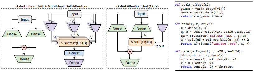
Gated Attention Unit (GAU)
핵심 아이디어는 attention과 GLU를 하나의 통합 layer로 만드는 것입니다. 그럼으로써 그 둘의 연산을 최대한 공유하게 하는 것입니다. 이는 연산 효율성 뿐만 아니라, attentive gating mechanism을 자연스럽게 강화합니다.
- $A \in \mathbb{R}^{T \times T}$ contains token-token attention weights
- $\hat{V} = AV$
GAU는 항상 $v_i$를 $u_i$의 gating에 사용한 GLU와 다르게 더욱 그럴듯한 representation인 $\hat{v}i = \sum_j a{ij}v_j$ 를 사용합니다. 만약 A가 identity matrix라면, GAU는 GLU와 동일해집니다.
gating 기법을 사용하면 MHSA 대비 훨씬 간단한 attention mechanism을 quality loss 없이 적용할 수 있습니다.
Z가 공유되는 representation $(s « d)^3$ 일 때, $\mathcal{Q}$는 per-dim scalars을 적용하고 $\mathcal{K}$는 offsets to Z를 해주는 가성비 좋은 변환입니다. b는 relative position bias입니다. 또한 MHSA의 softmax가 GAU의 경우 일반 활성화 함수로 단순화될 수 있음을 발견했습니다.
Transformer의 MHSA가 $4d^2$의 parameters가 필요한데 반해, GAU의 attention은 하나의 matrix인 $W_z$만을 필요로 하고 이는 $ds$ parameters만 필요합니다. GAU에서 $e = 2d$로 설정하면, 모델 사이즈와 학습 속도를 유지하면서도 Transformer block (MLP/GLU + MHSA)를 두 개의 GAUs로 대체할 수 있습니다.
GAU vs. Transformer
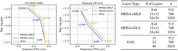
아래 Figure 3를 보면 GAUs가 Transformer block (MLP/GLU + MHSA)과 유사함을 확인할 수 있습니다. 아래 실험들은 상대적으로 짧은 context size(512)에서 진행됐음을 고려해야 합니다.
3. Fast Linear Attention with GAU
3.1. Existing Linear-Complexity Variants
Partial Attention
인기있는 방법들의 종류는 full attention matrix를 근사하려 했습니다.
- local window (Dai et al., 2019; Rae et al., 2019)
- local+sparse (Child et al., 2019; Li et al., 2019; Beltagy et al., 2020; Zaheer et al., 2020)
- axial (Ho et al., 2019; Huang et al., 2019)
- learnable patterns through hashing (Kitaev et al., 2020)
- clustering (Roy et al., 2021)
full attention만큼 효과적이진 않았지만, 이러한 변형들을 통해 longer sequences에서 대개 더 좋은 결과를 얻을 수가 있었습니다. 그러나 핵심적인 문제는 이러한 방법들이 GPU/TPU 병렬화에 도움이 되지 않는 memory re-formatting operations(gather, scatter, slice, concatenation)를 사용한다는 것입니다. 그래서 본 연구에서는 memory re-formatting operations을 최소화하기 위해 노력했습니다.
Linear Attention
한편으로는 attention matrix를 decomposing하고 matrix multiplications의 순서를 재배열하여 선형화 하려는 시도들이 있었습니다.
\[\hat{V}_{lin} = Q(K^{\top}V) \to \hat{V}_{quad} = softmax(QK^{\top})V\]또 다른 linear attention의 desirable property는 inference 때의 일정한 computation and memory 사용이었습니다.
\[M_t = M_{t-1} + K_tV_t^{\top}\]이것은 $O(d^2)$ 만큼의 캐시만 유지하면 된다는 의미입니다. 언제든 새로운 input이 들어왔을 때, $O(d^2)$ 만큼의 연산만 새로은 $M_t$를 얻기 위해 필요합니다. 그러나 decoding step에서는 full quadratic attention이 필요합니다.
그러나 re-arranging the computation in linear attention은 autoregressive training 과정에서 매우 큰 비효율을 보여줍니다. auto-regressive training에서 query vector $Q_t$는 다른 캐시 값인 $M_t$와 연관됩니다. 그러므로 모델은 총 T 개의 서로 다른 캐시 값 ${M}^T_{t=1}$ 을 준비해야 하는 것입니다. 이는 non-autoregressive case에서 $K^{\top}V$ 하나의 값만 필요한 것과 대비됩니다.
이론적으로는 sequence ${M}^T_{t=1}$는 첫 ${K_tV_t^{\top}}^T_{t=1}$ 연산으로부터 $O(Td^2)$만에 얻어질 수 있고, 누적 합 (cumsum) 연산을 T 토큰들에 대해 수행할 수 있습니다. 그러나 실제로는 “cumsum” 연산이 RNN-style의 T step에 대한 sequential dependency를 갖고 있으므로 매 스텝마다 $O(d^2)$ state가 필요합니다. 이러한 sequential dependency는 병렬화를 어렵게 만들 뿐만 아니라, 메모리에 T번 접근하게 만듭니다.
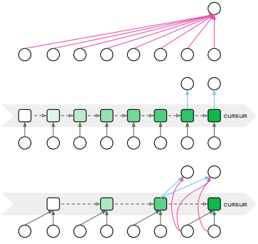
3.2. Our Method: Mixed Chunk Attention
지금까지의 linear-complexity attentions의 강점과 약점을 바탕으로 mixed chunk attention을 제안합니다.
Preparation
- The input sequence는 우선 서로 겹치지 않게 size $C$의 크기로 나누어 $G$를 생성합니다.
- 그리고 $U_g \in \mathbb{R}^{C \times e}$, $V_g \in \mathbb{R}^{C \times e}$, $Z_g \in \mathbb{R}^{C \times s}$를 GAU 수식에 따라 각 chunk에 대해 생성합니다.
- 그리고 네 개의 attention heads $Q_g^{quad}, K_g^{quad}, Q_g^{lin}, K_g^{lin}$를 $Z_g$로부터 per-dim scaling과 offset을 적용해서 생성합니다.
Local attention per chunk
우선 local quadratic attention은 독립적으로 각각의 길이 $C$인 chunk에 대해 적용됩니다.
\[\hat{V}_g^{quad} = relu^2(Q_g^{quad}, {K_g^{quad}}^{\top} + b) V_g\]위 수식의 복잡도는 $O(G \times C^2 \times d) = O(TCd)$ 입니다.
Global attention across chunks
global linear attention mechanism은 chunks 간의 long-range 상관관계를 도출합니다.
위의 두 시식이 chunk level에서 수행된다는 사실에 유의해야 합니다. 일반적인 casual(auto-regressive) 상황에서 이것은 cumsum의 대상 숫자를 줄여줍니다. 최종적으로 $\hat{V}_g^{quad}, \hat{V}_g^{lin}$을 더해줍니다.
\[O_g = [U_g \odot (\hat{V}_g^{quad} + \hat{V}_g^{lin})]W_o\]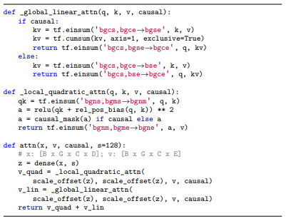
Fast Auto-regressive Training
chunking 덕분에 auto-regressive case에서의 sequential dependency가 T steps에서 G = T/C로 줄어들었습니다. 그 덕분에 auto-regressive training이 chunk size {128, 256, 512}에서 모두 비약적으로 빨라졌습니다. 그럼에도 일정한 per-step decoding memory와 computation을 유지할 수 있습니다.
On Non-overlapping Local Attention
FLASH에서 Chunks는 서로 겹치지 않습니다. 이론적으로는 꼭 겹치지 않을 필요는 없습니다. 이를 실험하고자 local attention overlapping을 허용해보기도 했습니다. 그럼에도 지속적으로 품질 향상을 보여줬지만, memory re-formatting operations들이 똑같이 필요해서 실제 실행 속도를 감소시켰습니다.
Connections to Combiner
FLASH와 비슷하게 Combiner (Ren et al., 2021) 또한 sequence를 nonoverlapping chunks로 분리했습니다. 가장 큰 차이점은 어떻게 long-range information을 요약하는지입니다. within each chunk. The key difference lies in how the longrange information is summarized and combined with the local information (e.g., our mixed chunk attention allows larger effective memory per chunk hence leads to better quality). See Appendix A for detailed discussions.
4. Experiments
4.0 Baselines
standard baseline: the vanilla Transformer (Vaswani et al., 2017) with GELU (Hendrycks & Gimpel, 2016)
- Transformer+: Transformer + RoPE (Su et al., 2021)
- Transformer++: Transformer + RoPE (Su et al., 2021) + GLU (Shazeer, 2020)
Linear complexity Transformer variants
- Performer (Choromanski et al., 2020): ReLU-kernel variant of Performer + RoPE
- Combiner (Ren et al., 2021): the rowmajor-axial variant of Combiner + RoPE
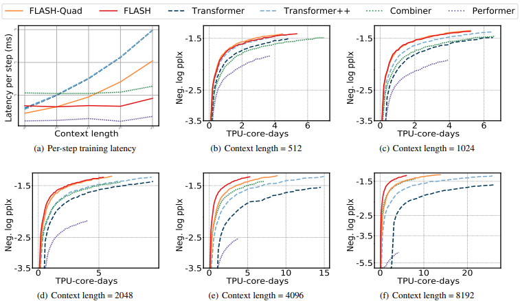
4.1. Bidirectional Language Modeling
masked language modeling (MLM)은 임의의 삭제된 tokens를 복원하는 태스크입니다. 모든 모델들의 pretrain and evaluate에는 C4 dataset (Raffel et al., 2020)을 사용했습니다.
- train each model with $2^{18}$ tokens per batch for 125K steps
- context length {512, 1024, 2048, 4096, and 8192}
- perplexity as a proxy metric
- 학습 속도는 “64 TPU-v4 cores”로 측정, “TPU-v4-core-days”로 기록
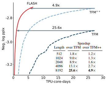
실험 결과는 다음과 같습니다.
- Context length가 커짐에 따라 FLASH, Combiner, Performer는 거의 일정한 모습을 보여줌
- FLASH-Quad도 느리지만 baselines 보다는 빠른 결과를 보여줌
- perplexity 기준으로 FLASH가 가장 좋은 성능을 보여줌
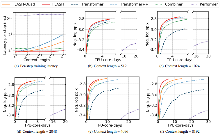
4.2. Auto-regressive Language Modeling
Auto-regressive Language Modeling에서는 Wiki-40B (Guo et al., 2020), PG-19 (Rae et al., 2019) datasets을 사용했습니다.
- train each model with $2^{18}$ tokens per batch for 125K steps
- context length
- Wiki-40B: {512, 1024, 2048, 4096, and 8192}
- PG-19: {1024, 2048, 4096, and 8192}
실험 결과는 다음과 같습니다.
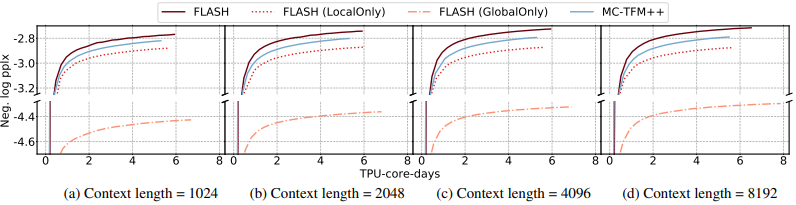
4.3. Ablation Studies
Significance of quadratic & linear components
“local quadratic attention”과 “global linear attention” 각각의 performance 기여분을 테스트 했습니다. 서로 상호 작용을 하며 중요한 역할을 한다는 것을 아래와 같이 확인했습니다.
Significance of GAU
FLASH에 있어 GAU의 중요성을 테스트 했습니다. 이를 위해 Transformer++에 mixed chunk attention을 적용했습니다.
Impact of chunk size
chunk size는 quality와 training cost 둘 다에 큰 영향을 줍니다. 일반적으로 context length가 길어짐에 따라 큰 chunk 크기를 적용할 때 더 좋은 결과를 보여주는 것을 확인했습니다.